| Variable | Frequency | Mean | SD | Minimum | Maximum |
|---|---|---|---|---|---|
| Importer | 826,499 | ||||
| Exporter | 826,499 | ||||
| Year | 826,499 | 2007 | 2021 | ||
| Soybean (USD '000) | 826,499 | 3,409.964 | 250,771.413 | 0.000 | 65,795,861.388 |
| Soy oil (USD '000) | 826,499 | 1,029.771 | 77,272.982 | 0.000 | 24,675,478.140 |
| Soy cake (USD '000) | 826,499 | 474.641 | 13,551.794 | 0.000 | 2,162,100.777 |
| Distance (KM) | 826,499 | 8,481.514 | 4,714.284 | 0.000 | 19,904.000 |
| Contiguity | 826,499 | 0.012 | 0.108 | 0.000 | 1.000 |
| Common language | 758,926 | 0.173 | 0.378 | 0.000 | 1.000 |
| Common colony | 758,926 | 0.118 | 0.323 | 0.000 | 1.000 |
| Soybean tariff | 826,499 | 0.064 | 0.414 | 0.000 | 7.574 |
| Soy oil tariff | 826,499 | 0.090 | 0.156 | 0.000 | 1.900 |
| Soy cake tariff | 826,499 | 0.035 | 0.075 | 0.000 | 0.715 |
The Possible Impact of EU Market Access Restrictions on the Soybean Trade and Deforestation
Manoj Sharma
Outline
- Motivation
- Method: Standard Gravity Framework
- Data
- Estimation: gravity model
- Simulation of EUDR implementation: setting
- Simulation of EUDR implementation: results and discussion
- Conclusion
Motivation: Trade and Deforestation
Trade causes deforestation (Abman & Lundberg, 2020; Pendrill et al., 2019, Faria & Almeida, 2016; Tsurumi & Managi, 2012); teleconnections between geographically separated locations of consumption and production (Henders and Ostwald, 2014; Rulli et al. 2019)
However, whether trade policies can be leveraged to curb deforestation while meeting global food demand ? How trade motivate conservation ?
Existing literature purposes two distinct measures: demand-side measures and supply-side measures
Demand-side measures
- Trade restrictions, e.g. EUDR; Standards & certifications; Voluntary moratoria; FSC certification; Rainforest Alliance
Supply-side measures:
- Strenthening legal framework in producer countries, e.g. EU REDD+; Payment to Ecosystem Services (PES); Forest Code e.g. Brazil
Motivation: Trade restrictions
- Motivation for trade restriction: Climate Club Theory (Nordhaus, 2015)
- A coalition of countries can cooperate to penalize on non-compliant countries
- Trade relationships could serve as a means for demanding environmental actions from trading partners to alleviate potential negative externalities (Harstad, 2024a).
- Environmental actions -> “Not FTA, CTA” - making tariffs contingent on forest cover (Harstad 2024a, Harstad 2024b)
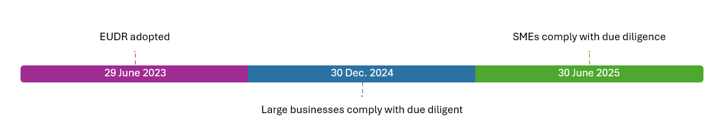
- Most recent example: EUDR
![]()
Source: Own illustration
Motivation: Question
(1) Can market access restriction by the EU eliminate deforestation from soy trade ?
Motivation: Why soybean?
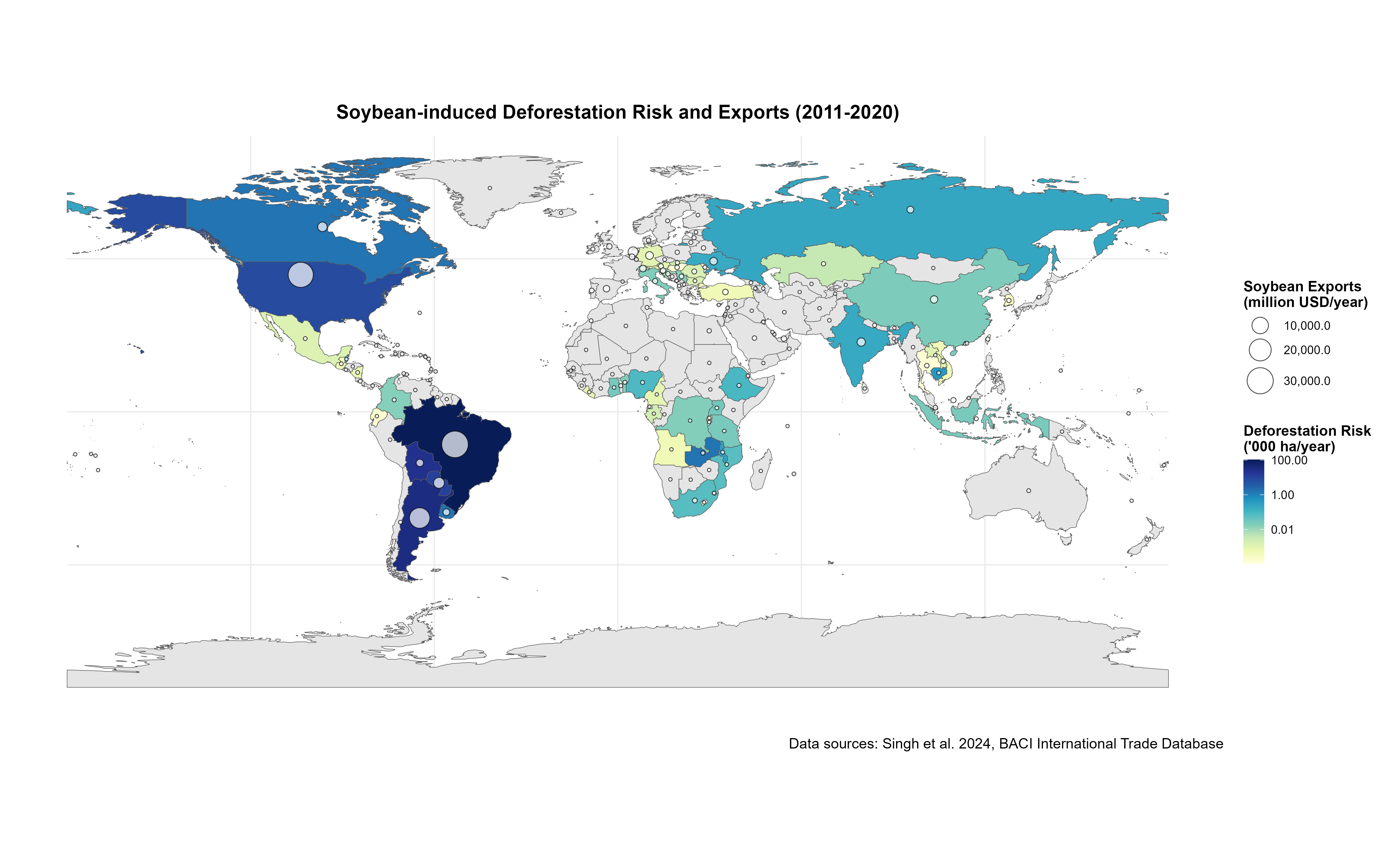
- Eliminating deforestation from export of Brazilian soy to the EU or China from 2011-2016 could have reduced net global deforestation by 2% and Brazilian deforestation by 9% (Villoria et al. 2022)
![]()
Motivation: EU trade and deforestation footprint
The EU is the world’s second-largest importer of soybeans, accounting for 9.88% of global exports,
Largest importer of soybean meals - which shares 23.82% of global soy trade - with approximately 24% of global exports (Comtrade, 2024).
The EU’s consumption accounts for 32.80 % of the deforestation associated with soybean production (Pendrill et al. 2019; European Parliament and of the Council 2023).
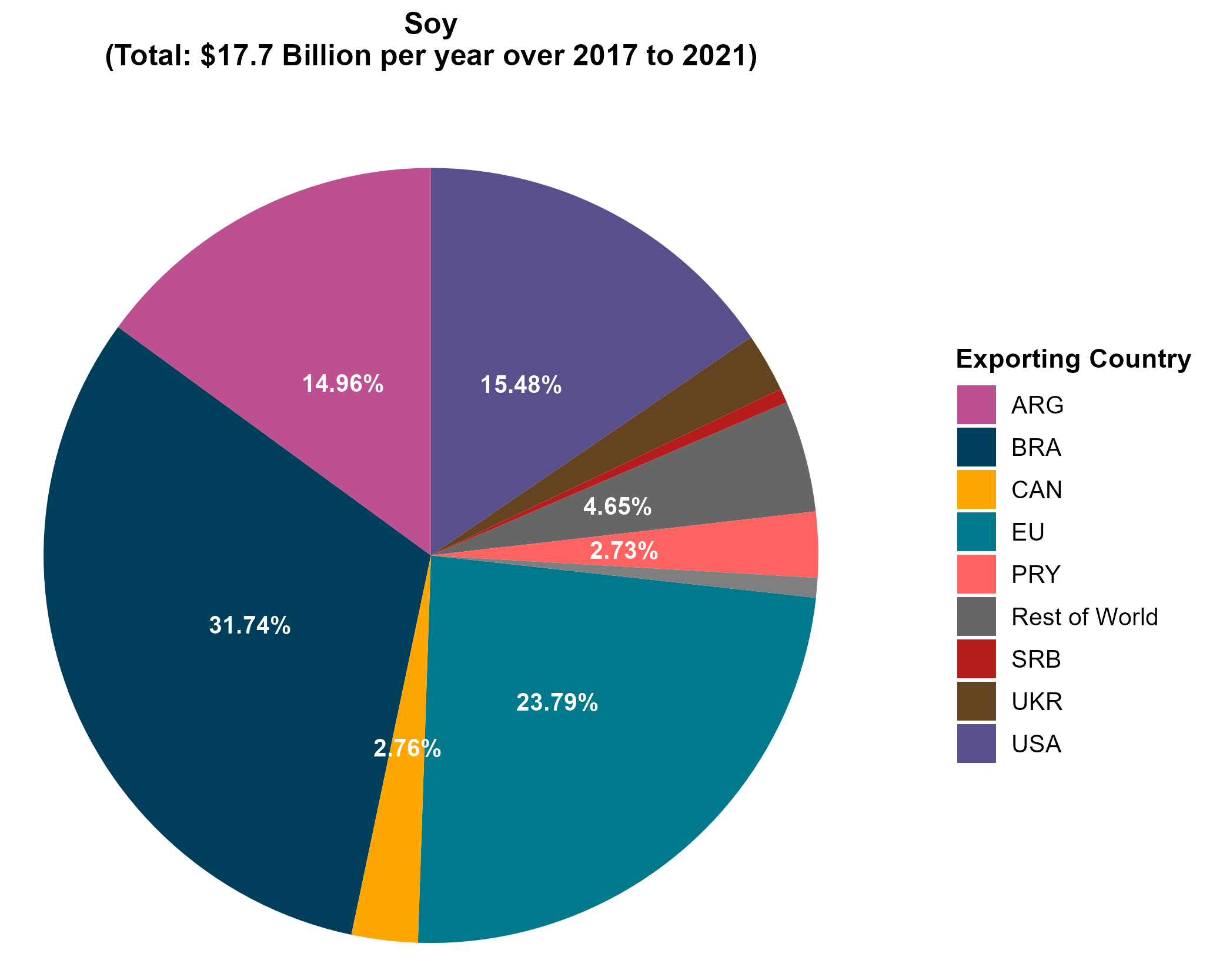
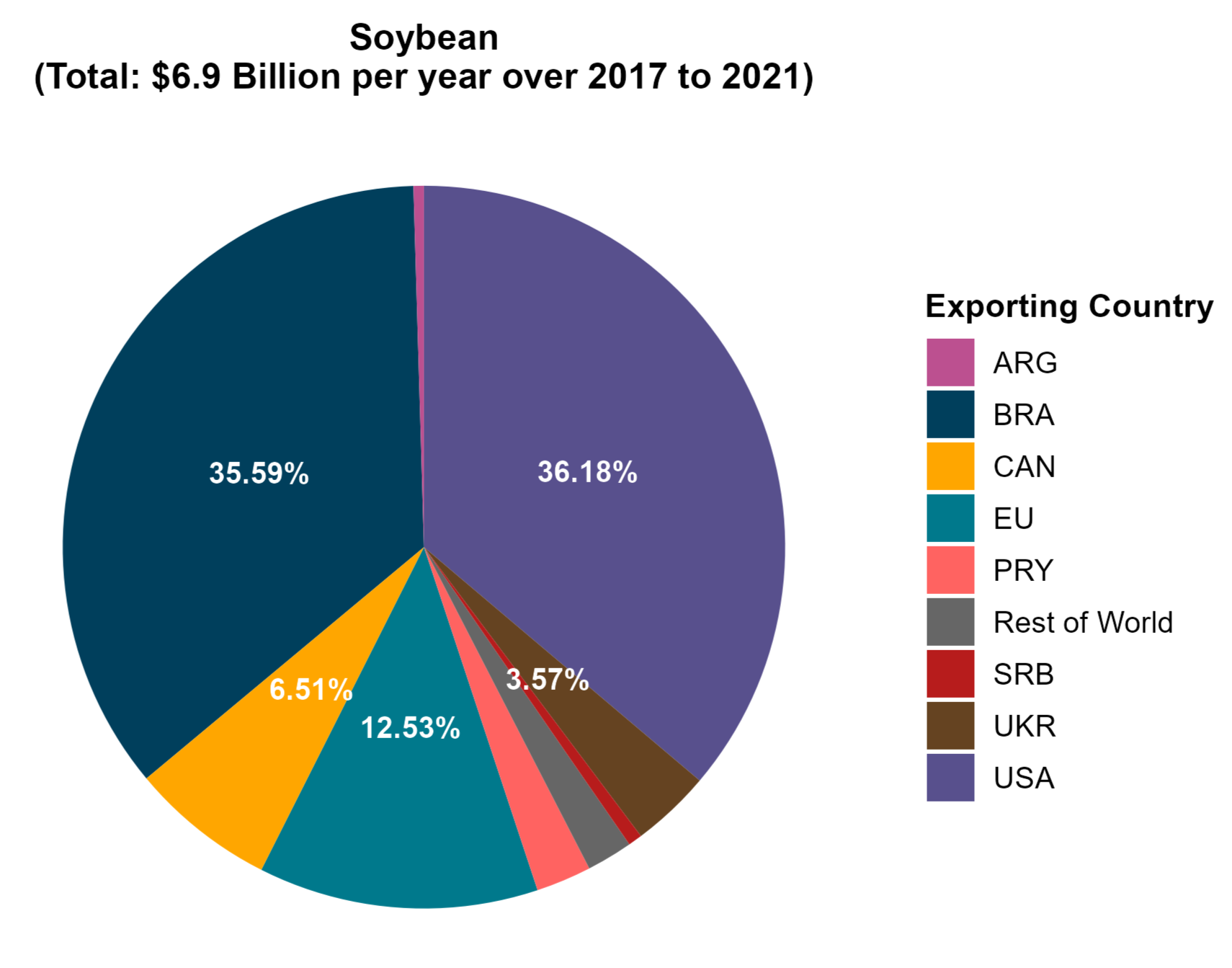
Motivation: EU soy trade
Method
- Two-stage estimation process
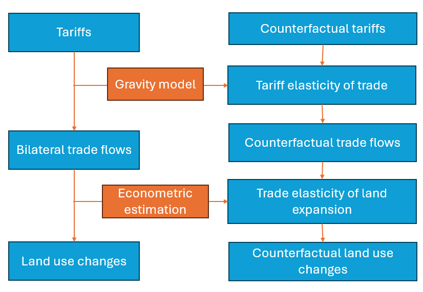
Figure 1. Estimation method to measure effectiveness of trade restrictions
Source: Own elaboration
Gravity Model: Theory
- Following the seminal work of Anderson (1979) and Anderson and Van Wincoop (2003), the bilateral trade flows is the function of the economic size and the trade cost between two countries.
Gravity Model: Econometrics counterpart
- Following the Silva and Tenreyro (2006), the equation (1) is expressed in its multiplicative form as:
\(\exp(\alpha_{ij} + \sum_{k=1}^{n} \alpha_k d_{k,ijt})\) is a counterpart of \((t_{ijt})^{1-\sigma}\), where \(\exp(\alpha_{ij})\) represents time-invariant bilateral trade costs and \(d_{k,ijt}\) represents time-varying bilateral trade costs
\(\exp(\alpha_{it})\) and \(\exp(\alpha_{jt})\) are exporter-time fixed effects and importer-fixed effects that captures OMR and IMR
Data
- Trade flow: CEPII-BACI (Gaulier & Zignago, 2010)
- Advantage: the reconciliation of mirror figures at product-level
- Domestic sales: FAOSTAT food balance database (FAOSTAT, 2024)
- Tariff: ITC-Market Access Map (2007- 2021) (ITC, 2024)
- Advantage: the consistent data on effectively applied tariffs
- Distance, Common language, Common colony, Contiguity: CEPII-Gravity database (Conte et al. 2022)
- Concordance between HS and FCL
- HS 120100, 120110 & 120190: Soybean (FCL 236)
- HS 150710 & 150790 : Soy oil (FCL 237)
- HS 230400: Soy cake (FCL 238)
Descriptive statistics
Empricial gravity model
- Two empirical models:
\(X_{ijt}^s = \exp(\gamma_{it}^s + \gamma_{jt}^s + \gamma_{ij}^s + \gamma_1^s \log(1 + \tau_{ijt}^s)) \varepsilon_{ijt}^s \tag{5a}\)
\(X_{ijt}^s = \exp(\gamma_{it}^s + \gamma_{jt}^s + \gamma_1 \log(1 + \tau_{ijt}^s) + \gamma_2 \log(\text{DIST}_{ij}) + \gamma_3 \text{CLNY}_{ij}\)
\(+ \gamma_4 \text{LANG}_{ij} + \gamma_5 \text{CNTG}_{ij}) \varepsilon_{ijt}^s \tag{5b}\)
where, \(s\in\) {soybean, soybean oil, soybean cake, soy}
- inclusion of distance \((DIST_{ij})\), colonial \((CLNY_{ij})\), common official language \((LANG_{ij})\) and contiguity \((CNTG_{ij})\) is motivated by the study of Borchert et al. (2021)
Result: tariff elasticity of trade
Table 2. Effects of tariffs on the soybean industry
Specification 5(a)
|
Specification 5(b)
|
|||||||
|---|---|---|---|---|---|---|---|---|
| Variables | (1) | (2) | (3) | (4) | (5) | (6) | (7) | (8) |
| Gravity Variables | ||||||||
| Log tariff | -7.60** (3.08) | -5.73** (2.38) | -12.4*** (4.53) | -2.50*** (0.75) | -6.53*** (1.96) | -15.6*** (2.13) | 3.59 (6.71) | -4.34*** (1.17) |
| Log distance | -2.28*** (0.09) | -1.88*** (0.06) | -0.66*** (0.14) | -1.77*** (0.05) | ||||
| Contiguity | -0.56** (0.27) | -0.38* (0.20) | 1.71*** (0.32) | -0.26 (0.22) | ||||
| Common language | 0.04 (0.29) | -0.20 (0.20) | 0.40 (0.26) | -0.02 (0.21) | ||||
| Common colony | -0.76 (0.93) | -1.07* (0.60) | 1.02** (0.40) | 0.08 (0.34) | ||||
| Fixed Effects | ||||||||
| Fixed-Effects | ||||||||
| Importer-Year | ✓ | ✓ | ✓ | ✓ | ✓ | ✓ | ✓ | ✓ |
| Exporter-Year | ✓ | ✓ | ✓ | ✓ | ✓ | ✓ | ✓ | ✓ |
| Country pairs | ✓ | ✓ | ✓ | ✓ | ✗ | ✗ | ✗ | ✗ |
| Model Statistics | ||||||||
| Observations | 42,223 | 44,539 | 31,006 | 110,468 | 397,720 | 489,081 | 425,150 | 557,000 |
| Squared Cor. | 0.999 | 0.999 | 0.961 | 0.998 | 0.991 | 0.996 | 0.534 | 0.987 |
| Pseudo R2 | 0.997 | 0.995 | 0.964 | 0.993 | 0.982 | 0.970 | 0.839 | 0.968 |
Note: ***, ** and * denotes below 1%, 5% and 10% significance, respectively.
Counterfactual exercise: setting
- Followed the steps developed by Anderson et al. (2018)
Step I: Conduct baseline gravity
\(X_{ijt} = \exp({\hat\gamma_1}\log(1+\tau_{ijt}) + \hat\gamma_{it} + \hat\gamma_{jt} +\hat\gamma_{ij}) \tag{6}\)
- Now, we take the reference year of 2021 and estimate baseline trade cost and price indexes:
\([\hat{\Pi}_{i}^{1-\sigma}]^{BLN} = \frac{Y_i}{\exp(\hat{\gamma}_{i})} \times E_{0} \tag{7}\)
\([\hat{P}_{j}^{1-\sigma}]^{BLN} = \frac{E_j}{\exp(\hat{\gamma}_{j}) \times E_{0}} \tag{8}\)
- Many country-pairs have zero trade flows. For such country, \(\exp(\hat\gamma_{ij})\) are not available. Therefore, the following equation is estimated to predict \(\exp(\hat\gamma_{ij})\) for the missing country pair fixed effects.
\(\exp[\hat{\gamma_{ij}}] = \exp[\gamma_{i} + \gamma_{j} +\gamma_2lnDist_{ij} + \gamma_3CNTG_{ij} + \gamma_4LANG_{ij} + \gamma_5CLNY_{ij}]*\varepsilon_{ij} \tag{9}\)
Counterfactual exercise (cntd..)
Therefore, the baseline trade cost is estimated as below:
\([(t_{ij})^{1-\sigma}]^{BLN} = \begin{cases} \exp(\hat{\gamma}_{ij}) \exp(\hat\gamma_1\ln(1+\tau_{ij})) & \text{if } X_{ij} > 0 \text{ for at least one period} \\ \hat\exp(\hat{\gamma}_{ij})\exp(\hat\gamma_1\ln(1+\tau_{ij})), & \text{if }X_{ij} = 0\text{ for all period} \end{cases} \tag{10}\)
Step 2: Counterfactual construction
\([\hat{t}_{ij}^{1-\sigma}]^{CFL} = \exp[\hat{\gamma}_{ij} + \hat{\gamma}_1 \log(1+\tau_{ij}^{{CFL}})] \tag{11}\)
Counterfactual exercise (cntd..)
Step3: Estimate conditional gravity
\(X_{ij} = [\hat{t}_{ij}^{1-\sigma}]^{CFL}\exp[\gamma_{i}^{CFL} + \gamma_{j}^{CFL}]*\varepsilon_{ijt}^{CFL} \tag{12}\)
From the estimation of above equation, we estimate counterfactual price indexes as below:
\([\hat{\Pi}_{i}^{1-\sigma}]^{CFL} = \frac{Y_i}{\exp(\hat{\gamma}_{i}^{CFL})} * E_{0} \tag{13}\)
\([\hat{P}_{j}^{1-\sigma}]^{CFL} = \frac{E_j}{\exp(\hat{\gamma}_{j}^{CFL}) * E_{0}} \tag{14}\)
Thus, the counterfactual trade flow will be:
\(X_{ij}^{CFL} = [\hat{t}_{ij}^{1-\sigma}]^{CFL}\exp[\hat\gamma_{i}^{CFL} + \hat\gamma_{j}^{CFL}] \tag{15}\)
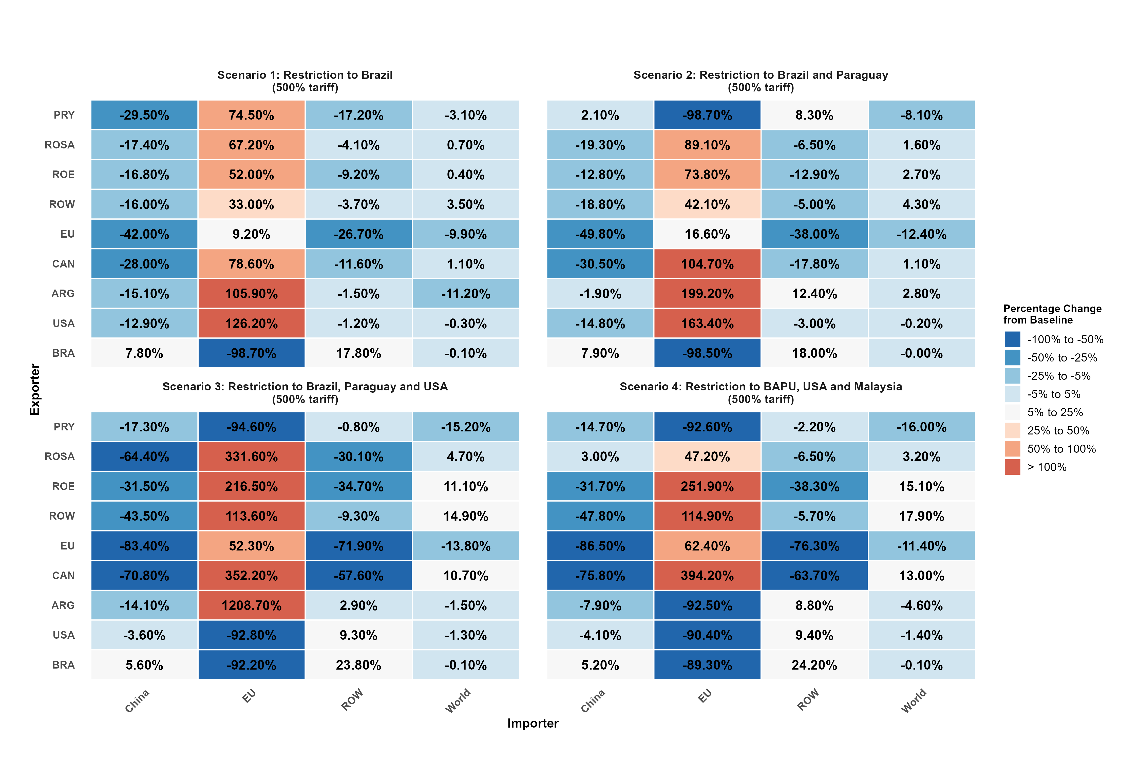
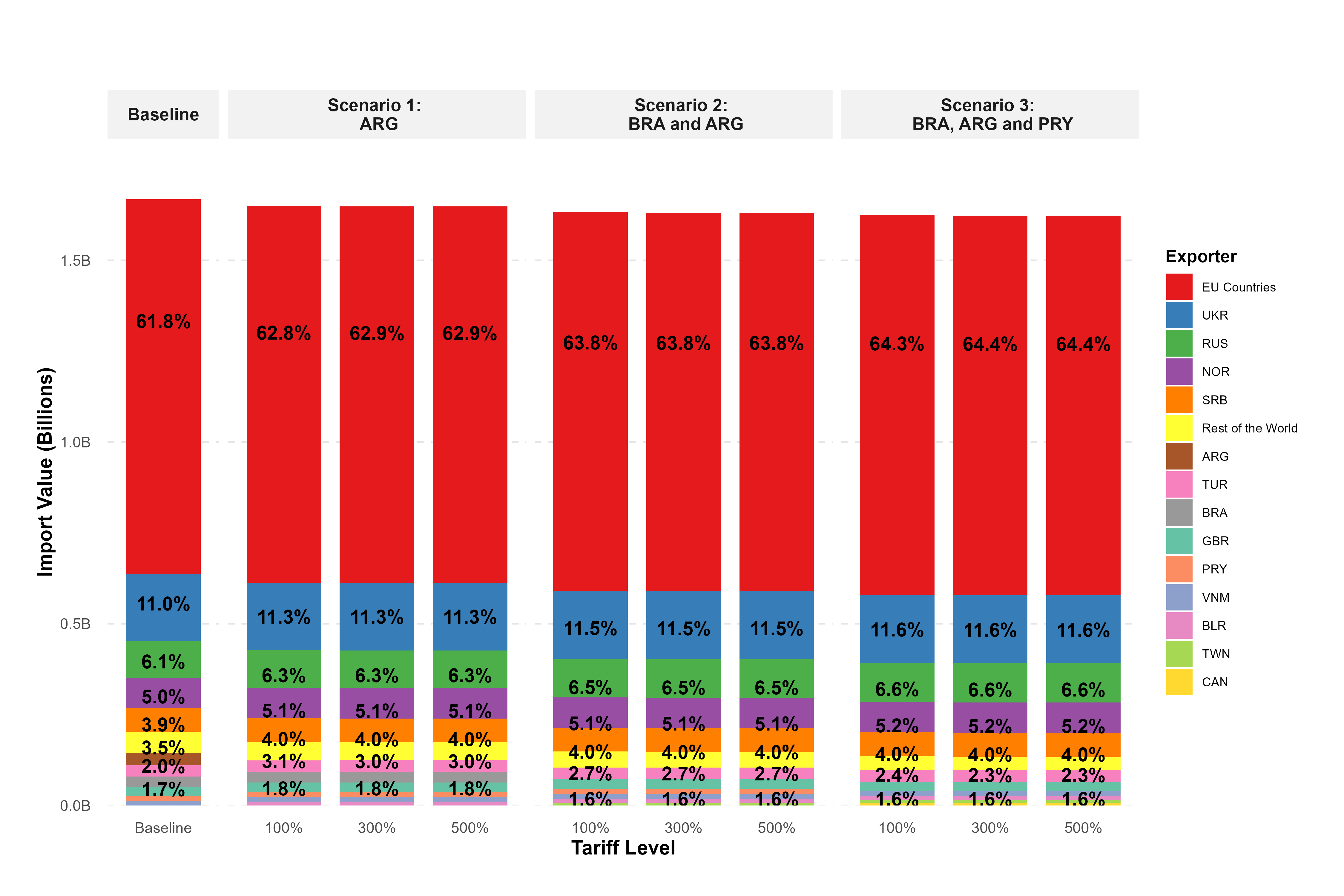
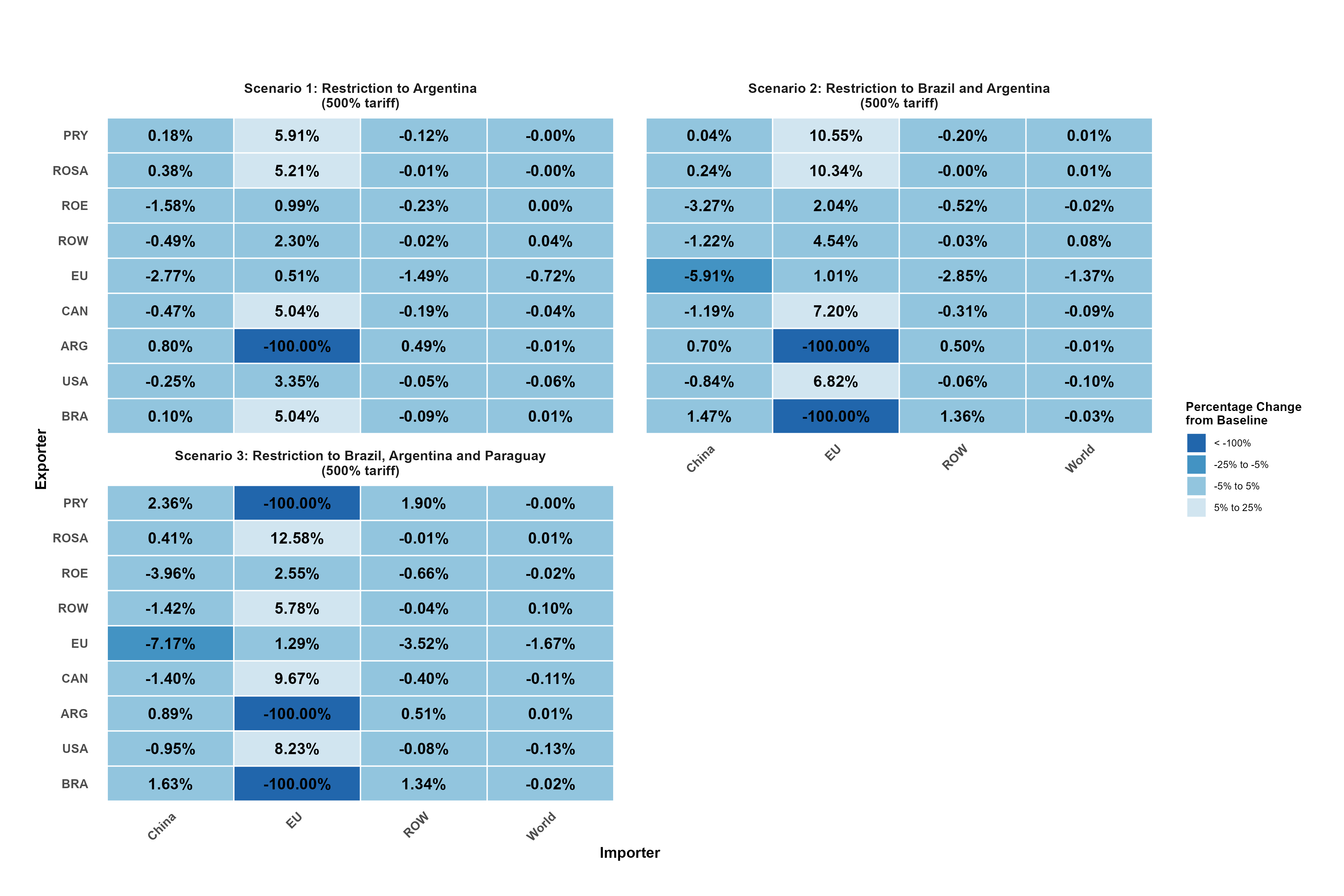
Counterfactual exercise: EUDR implementation
| Products | Scenario.I | Scenario.II | Scenario.III | Scenario.IV |
|---|---|---|---|---|
| Soybean | Trade restriction on Brazil (100%, 300% & 500%) |
Trade restriction on Brazil and Paraguay (100%, 300% & 500%) |
Trade restriction on Brazil, Paraguay and USA (100%, 300% & 500%) |
Trade restriction on Brazil, Argentina, Paraguay, Uruguay, USA and Malaysia (100%, 300% & 500%) |
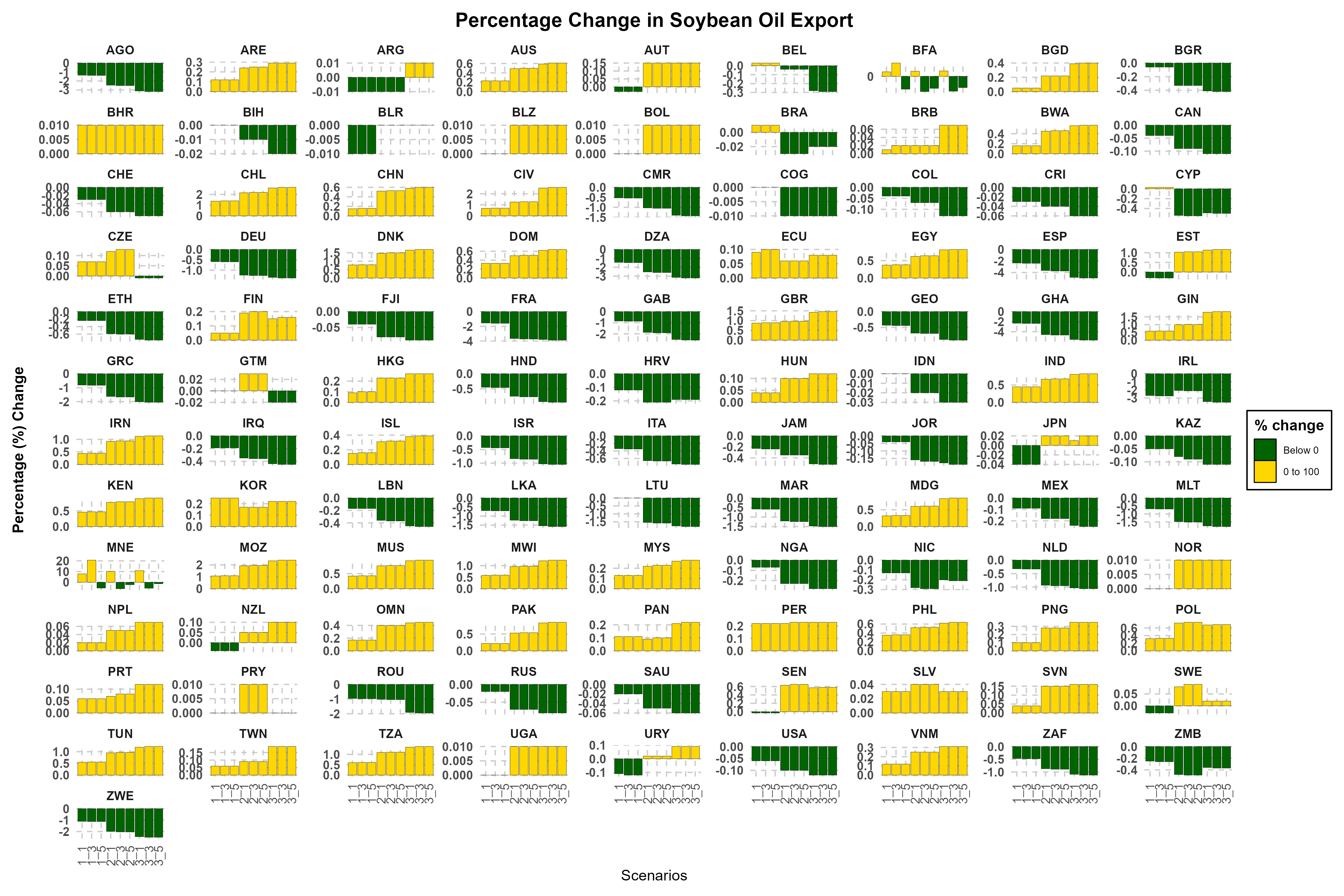
| Soybean oil | Trade restriction on Argentina (100%, 300% & 500%) |
Trade restriction on Brazil and Argentina (100%, 300% & 500%) |
Trade restriction on Brazil, Argentina and Paraguay (100%, 300% & 500%) |
|
| Soybean cake | Trade restriction on Brazil (100%, 300% & 500%) |
Trade restriction on Brazil and Argentina (100%, 300% & 500%) |
Trade restriction on Brazil, Argentina, Paraguay and Bolivia (100%, 300% & 500%) |
Trade restriction on Brazil, Argentina, Paraguay, Bolivia and USA (100%, 300% & 500%) |
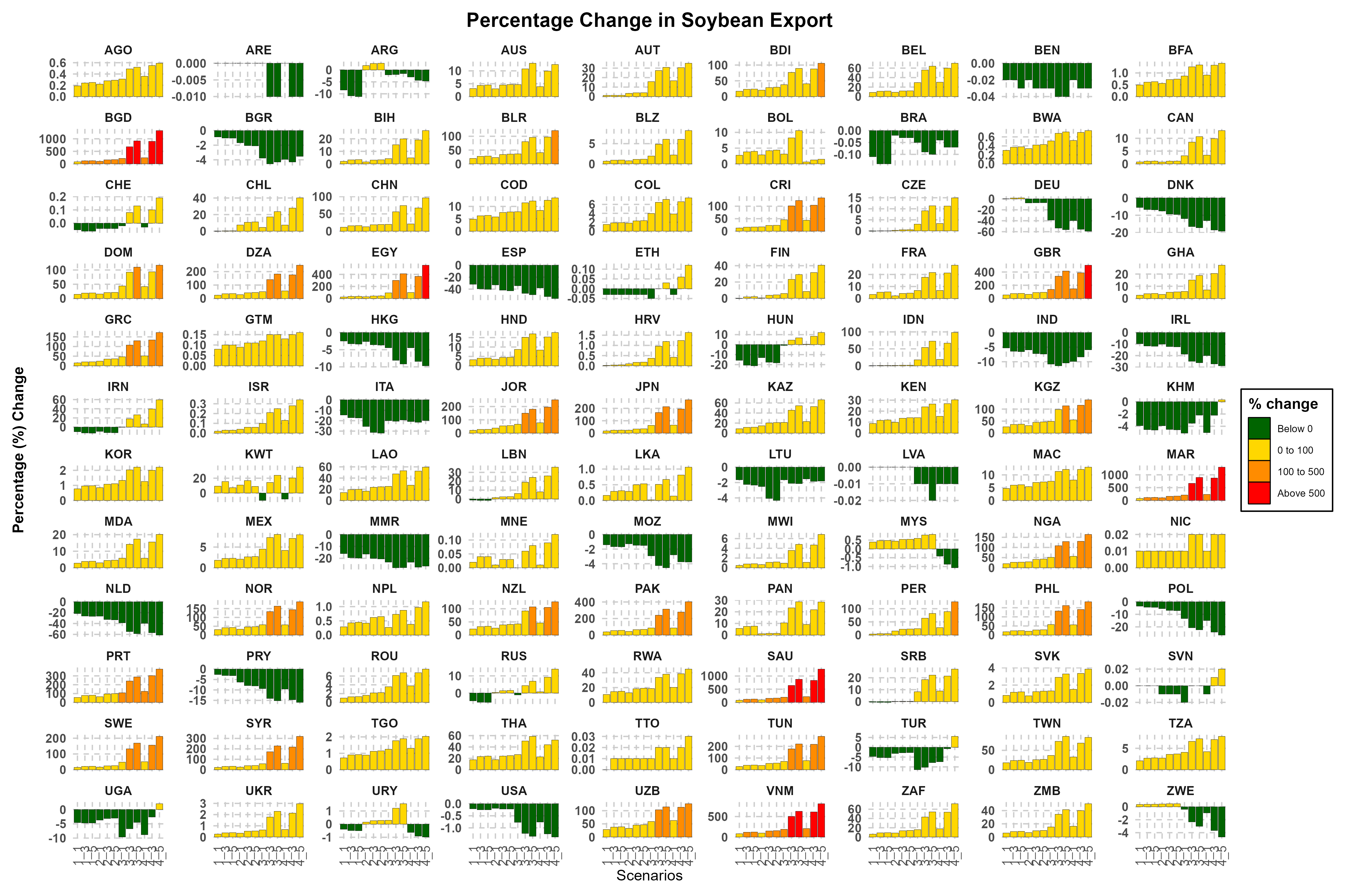
| Soy | Trade restriction on Brazil (300%, 500% & 1000%) |
Trade restriction on Brazil and Argentina (300%, 500% & 1000%) |
Trade restriction on Brazil, Argentina and Paraguay (300%, 500% & 1000%) |
Trade restriction on Brazil, Argentina, Paraguay and USA (300%, 500% & 1000%) |
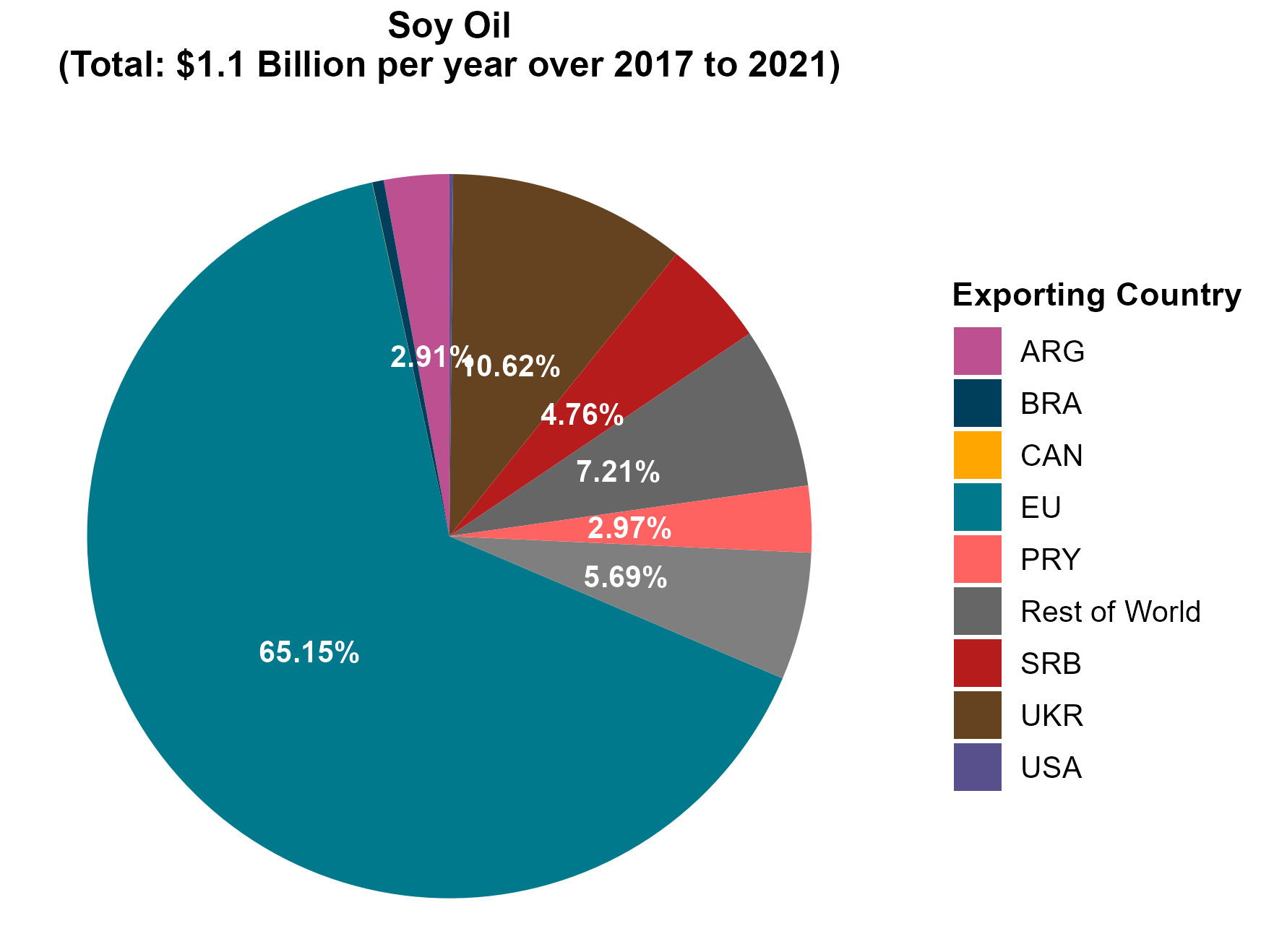
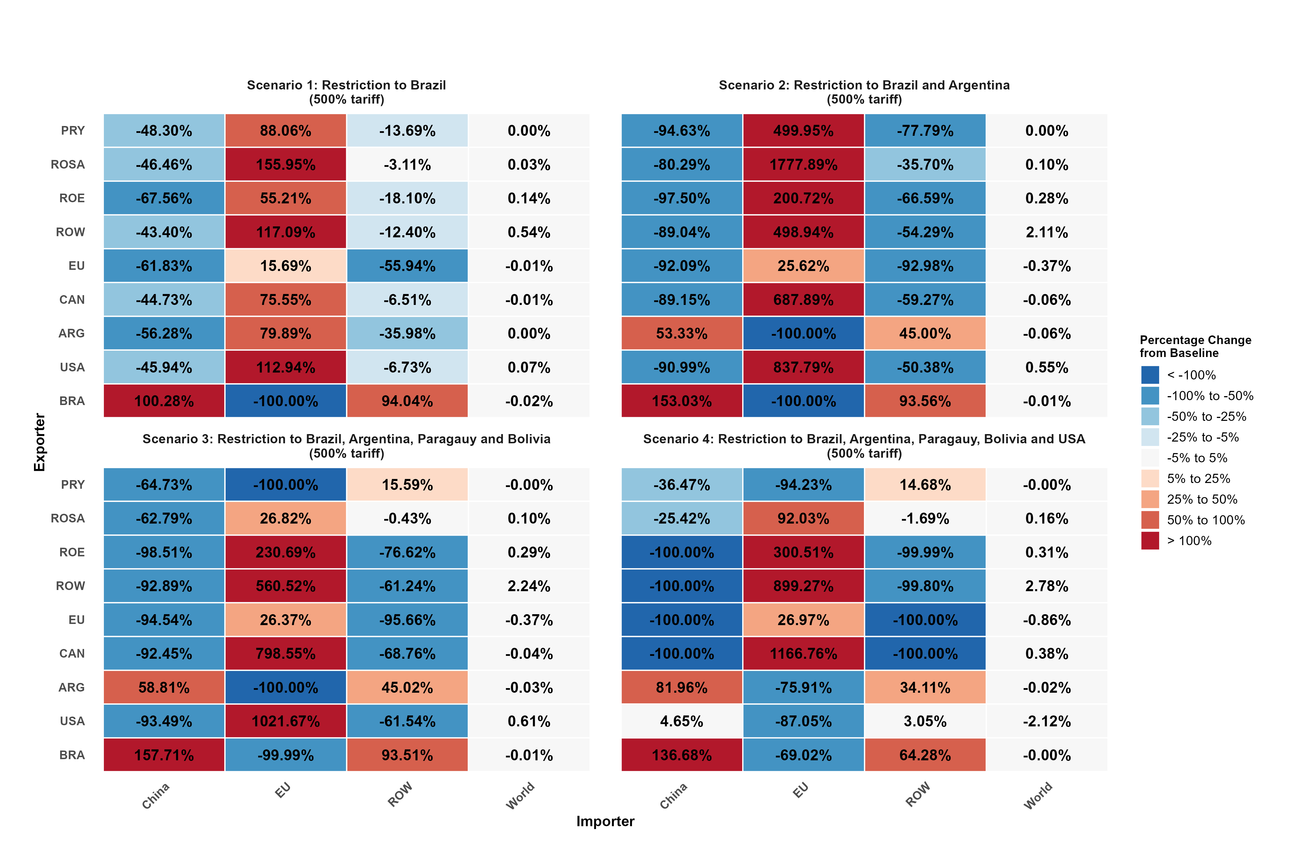
Counterfactual exercise: EU import in soybean
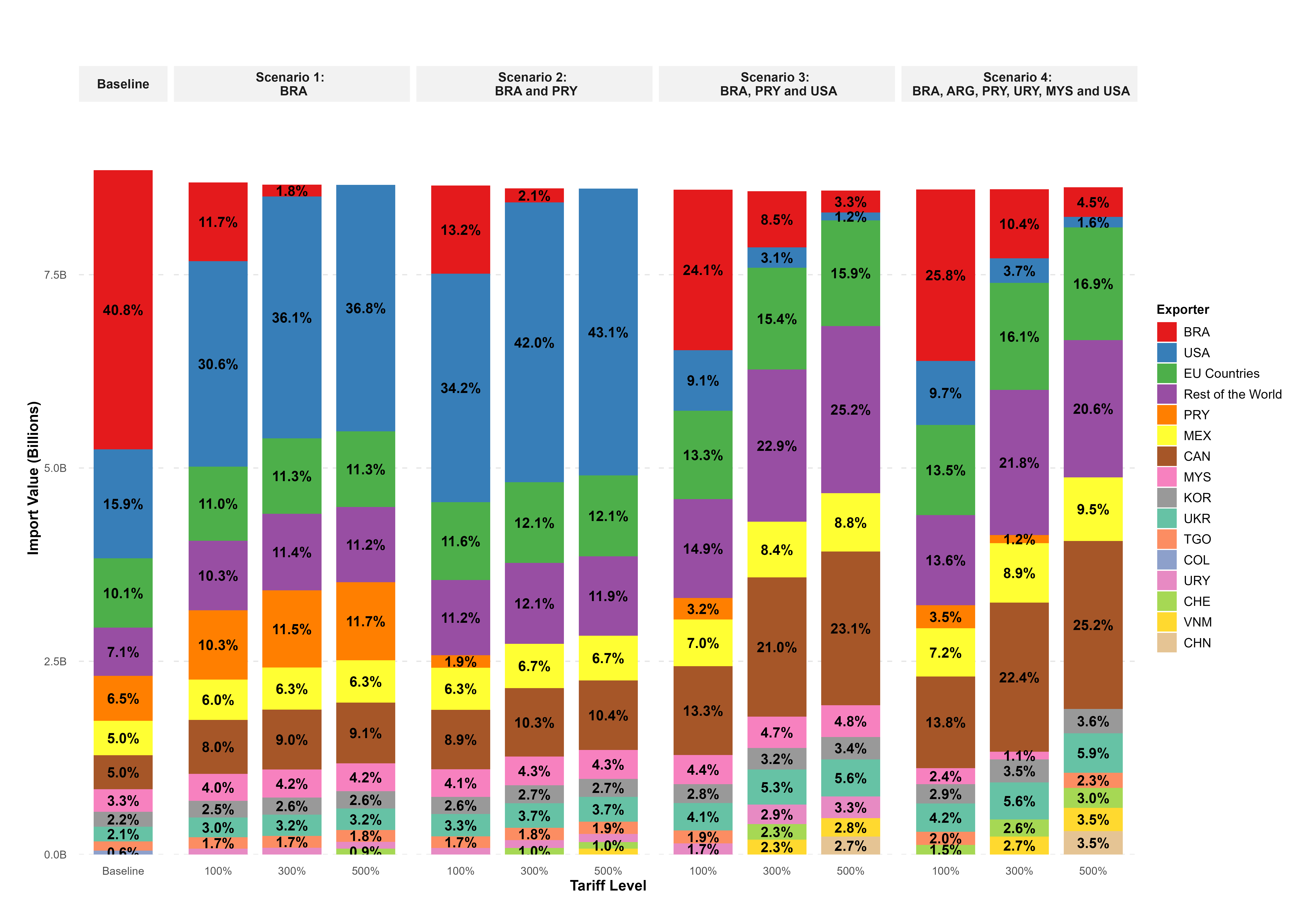
Counterfactual exercise: Trade diversion in soybean
Counterfactual exercise: EU import in soybean oil
Counterfactual exercise: Trade diversion in soybean oil
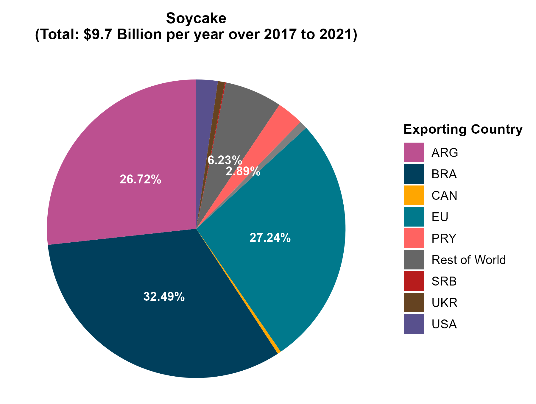
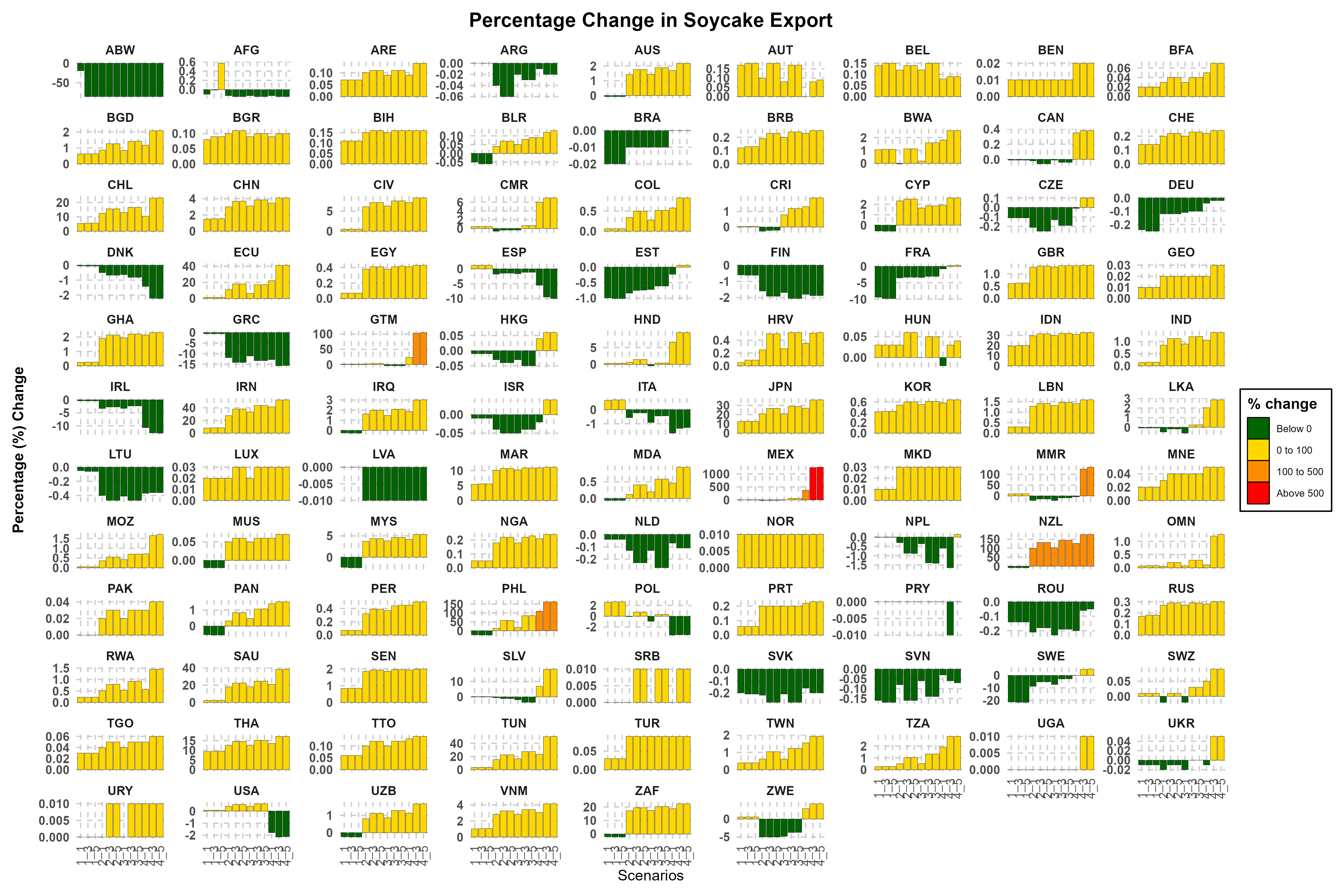
Counterfactual exercise: EU import in soybean cake
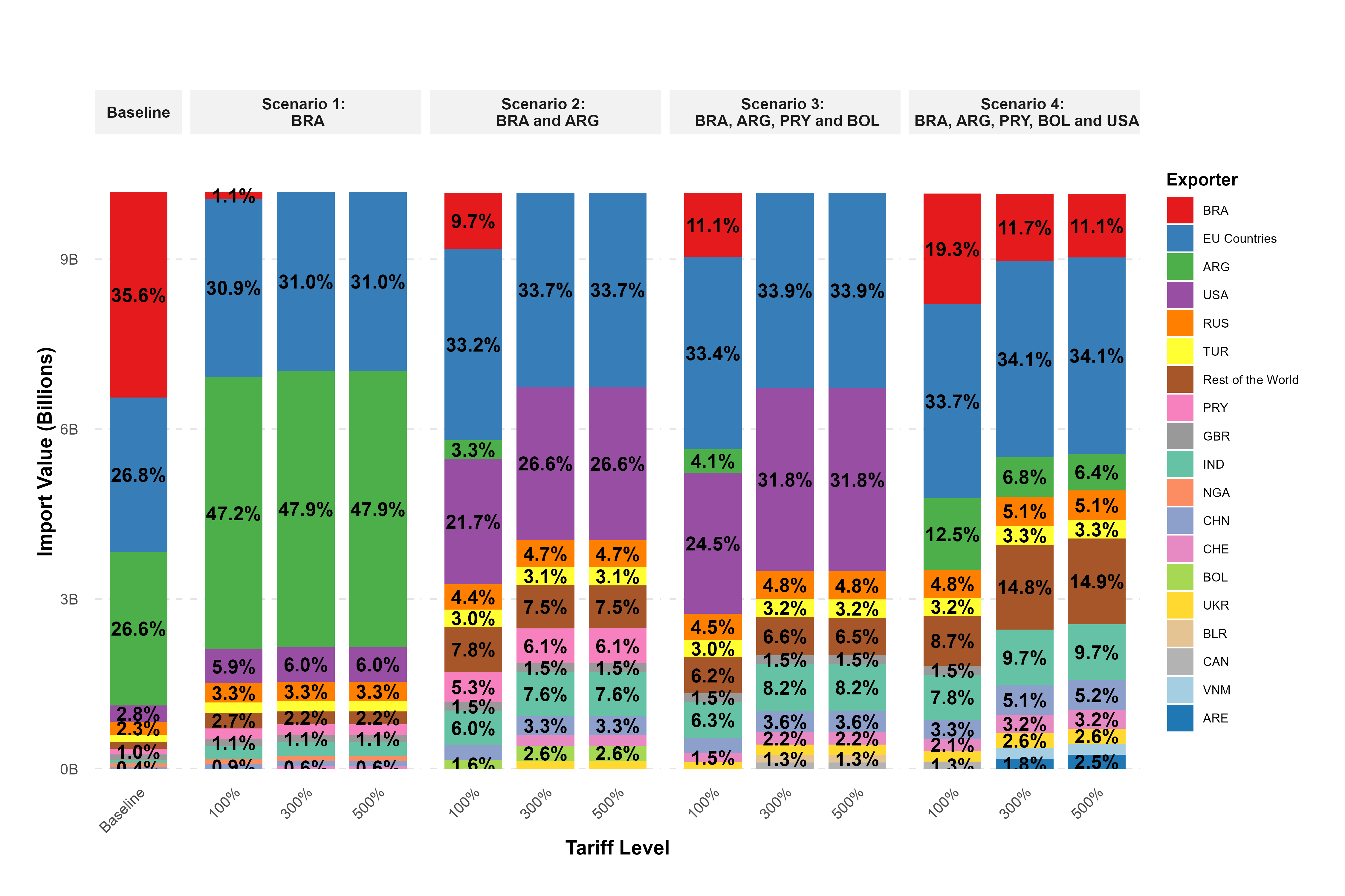
Counterfactual exercise: Trade diversion in soybean cake
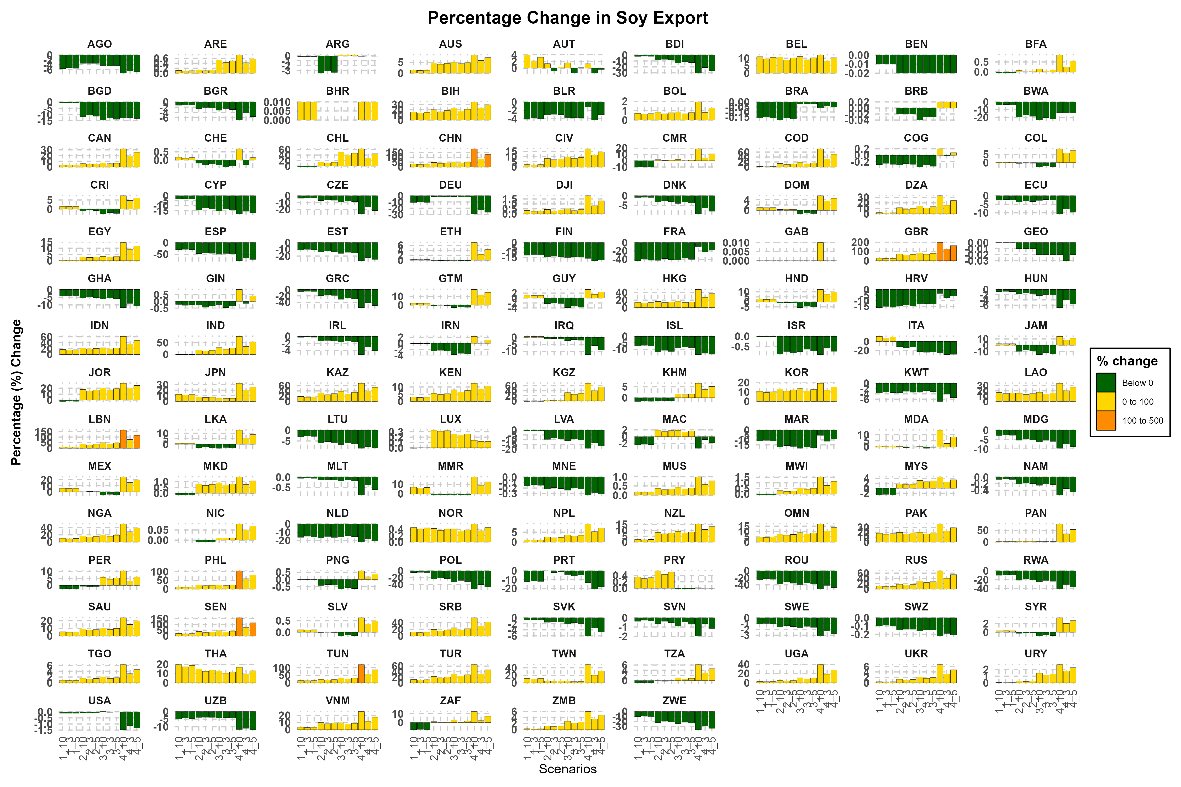
Counterfactual exercise: EU imports in soy
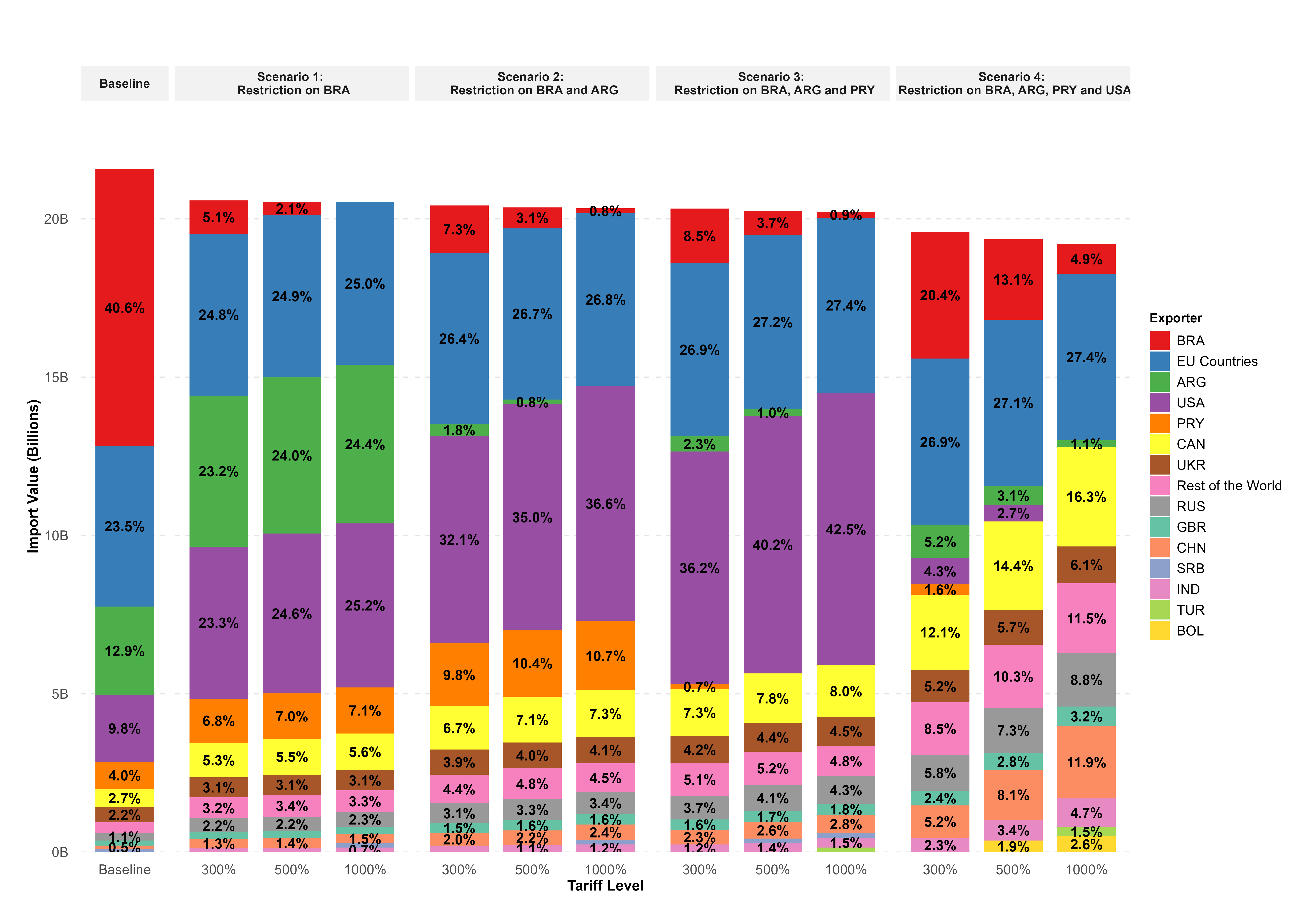
Counterfactual exercise: Trade diversion in soy

Conclusion
- Trade restriction by EU cannot restrict the exports from Brazil, Argentina and Paraguay significantly, and so is the deforestation
- However, the consumers in the EU may suffer
- Trade restriction by EU just redirects the export to China \(\implies\) redirection of the problem
- EUDR may possibly ineffective in soy industry
- USA, Canada and countries from Asia may get market opportunities
- The EU may need to consider alternative strategies, such as incentivizing forest conservation and enhancing cooperation with source countries.
References
- Henders, S., & Ostwald, M. (2014). Accounting methods for international land-related leakage and distant deforestation drivers. Ecological Economics, 99, 21-28.
- Rulli, M. C., Casirati, S., Dell’Angelo, J., Davis, K. F., Passera, C., & D’Odorico, P. (2019). Interdependencies and telecoupling of oil palm expansion at the expense of Indonesian rainforest. Renewable and Sustainable Energy Reviews, 105, 499-512.
- Abman, R., & Lundberg, C. (2020). Does free trade increase deforestation? The effects of regional trade agreements. Journal of the Association of Environmental and Resource Economists, 7(1), 35-72.
- Borchert, I., Larch, M., Shikher, S., & Yotov, Y. V. (2021). The international trade and production database for estimation (ITPD-E). International Economics, 166, 140-166.
- Gaulier, G., & Zignago, S. (2010). BACI: International Trade database at the product-level (the 1994-2007 version).CEPII Working Paper, N°2010-23. BibTex. https://www.cepii.fr/CEPII/en/bdd_modele/bdd_modele_item.asp?id=37
- ITC. (2024). Market Access Map. https://www.macmap.org/en/user-account/login-to-continue?ReturnUrl=%2fen%2fdownload (accessed on 23 August 2024) Conte, M., Cotterlaz, P., & Mayer, T. (2022). The CEPII gravity database. CEPII Working paper N°2022-05, July 2022. https://www.cepii.fr/CEPII/en/bdd_modele/bdd_modele_item.asp?id=8
- Singh, C., & Persson, U. M. (2024). Global patterns of commodity-driven deforestation and associated carbon emissions. EarthArXiV, Apr.
- FAO. (2024). FAOSTAT Food Balances. https://www.fao.org/faostat/en/#data
- Abman, R., & Lundberg, C. (2020). Does free trade increase deforestation? The effects of regional trade agreements. Journal of the Association of Environmental and Resource Economists, 7(1), 35-72.
- Faria, W. R., & Almeida, A. N. (2016). Relationship between openness to trade and deforestation: Empirical evidence from the Brazilian Amazon. Ecological Economics, 121, 85-97.
- Tsurumi, T., & Managi, S. (2014). The effect of trade openness on deforestation: empirical analysis for 142 countries. Environmental Economics and Policy Studies, 16, 305-324.
- Taheripour, F., Hertel, T. W., & Ramankutty, N. (2019). Market-mediated responses confound policies to limit deforestation from oil palm expansion in Malaysia and Indonesia. Proceedings of the National Academy of Sciences, 116(38), 19193-19199.
- Harstad, B. (2024a). Trade and trees. American Economic Review: Insights, 6(2), 155-175.
- Harstad, B. (2024b). Contingent Trade Agreements (No. w32392). National Bureau of Economic Research.
- Nordhaus, W. (2015). Climate clubs: Overcoming free-riding in international climate policy. American Economic Review, 105(4), 1339-1370.
- Pendrill, F., Persson, U. M., Godar, J., Kastner, T., Moran, D., Schmidt, S., & Wood, R. (2019). Agricultural and forestry trade drives large share of tropical deforestation emissions. Global environmental change, 56, 1-10.
Counterfactual exercise: winners and losers in soybean
Counterfactual exercise: winners and losers in soybean oil
Counterfactual exercise: winners and losers in soybean cake
Counterfactual exercise: winners and losers in Soy
Land Use Model: Theory
Land Supply: Assume that agricultural land \(L_i\) for soybean is supplied from two sources in each country, \(i\),: all agricultural productive land \(H_{i}\) and forest cover \(F_i\). In terms of relative change,
\[\begin{gather*} \small l_i^s = \theta_i^h h_i + \theta_i^f f_i \tag{5} \\ \end{gather*}\]where, \(\theta_i^h\) is agricultural land elasticity of soybean land, and \(\theta_i^f\) is forest cover elasticity of soybean land. For countries where soybean are forest risk commodities, \(\theta_i^f\) will be smaller.
According to Hertel (1989), there exists a relationship between relative land use and relative rental value such that, \(h_i = \nu_ir_i\).
Wide range of research suggest that change in forest cover is driven by government effectiveness, in particular property right. If property right is defined and domestic policy is pro-forestry, \(f_i\) is non-negative. Therefore, forest cover can be defined as \(F_i = F_i(\zeta_i)\), where \(\zeta_i\) is government effectiveness.
Let \(f_i = \delta_i\xi_i\)
Land Use Model: Theory
Land Demand: Following Villoria (2019), minimizing the cost of production subject to parsimonius CES production technology, yields the land demand as:
\[\begin{gather*} l_i^D = q_i - z_i - \phi_i[r_i - p_i - z_i] \tag{7} \\ \end{gather*}\]where,
- \(l_i^D\) is the relative change in land demand
- \(q_i\) is the relative change in output
- \(\phi_i\) is the elasticity of substitution between land and non-land factors
- \(z_i\) is the relative change in technology
- \(r_i\) is the relative change in land rent
- \(p_i\) is the relative change in price of output
Land Use Model: Theory
Equilibrium: Equation equations (6) & (7), we get
\[\begin{gather*} r_i^* = \frac{q_i - z_i + \phi_i[p_i + z_i] - \theta_i^f\delta_i\xi_i }{\theta_i^h\nu_i + \phi_i} \tag{8} \end{gather*}\]Equilibrium land use: Substituting equation equation (8) on equation (6), we get:
\[\begin{gather*} l_i^* = \frac{\theta_i^h \nu_i}{\theta_i^h\nu_i + \phi_i}q_i + \frac{(\theta_i^h \nu_i)(\phi_i -1)}{\theta_i^h\nu_i + \phi_i}z_i + \frac{(\theta_i^h \nu_i)\phi_i}{\theta_i^h\nu_i + \phi_i}p_i + \frac{\theta_i^f\delta_i\phi_i}{\theta_i^h\nu_i + \phi_i}\xi_i \tag{9} \end{gather*}\]since, total export = production - consumption (\(E_i = Q_i - C_i\)) implies that:
\[\begin{gather*} q_i = e_i(x_i -p_i) + (1-e_i)(d_i - p_i) = e_ix_i + (1-e_i)d_i - p_i \tag{10} \\ \end{gather*}\]Land Use Model: Theory
The optimal land use becomes:
\[\begin{gather*} l_i^* = \underbrace{\frac{\theta_i^h \nu_i}{\theta_i^h\nu_i + \phi_i}e_ix_i}_{\text{International demand effect}} + \underbrace{\frac{\theta_i^h \nu_i}{\theta_i^h\nu_i + \phi_i}(1- e_i)d_i}_{\text{Domestic demand effect}} + \underbrace{\frac{(\theta_i^h \nu_i)(\phi_i -1)}{\theta_i^h\nu_i + \phi_i}z_i}_{\text{Technology effect}} + \underbrace{\frac{(\theta_i^h \nu_i)(\phi_i-1)}{\theta_i^h\nu_i + \phi_i}p_i}_{\text{Price effect}} + \underbrace{\frac{\theta_i^f\delta_i\phi_i}{\theta_i^h\nu_i + \phi_i}\xi_i}_{\text{Property right effect}} \tag{11} \end{gather*}\]since, \(f_i = \delta_i\xi_i\)
\[\begin{gather*} f_i = \underbrace{\frac{\theta_i^h\nu_i + \phi_i}{\theta_i^f \phi_i}l_i^*}_{\text{Domestic land demand effect}} - \underbrace{\frac{\theta_i^h \nu_i}{\theta_i^f \phi_i}e_ix_i}_{\text{International demand effect}} - \underbrace{\frac{\theta_i^h \nu_i}{\theta_i^f \phi_i}(1- e_i)d_i}_{\text{Domestic demand effect}} - \underbrace{\frac{(\theta_i^h \nu_i)(\phi_i -1)}{\theta_i^f \phi_i}z_i}_{\text{Technology effect}} - \underbrace{\frac{(\theta_i^h \nu_i)(\phi_i-1)}{\theta_i^f \phi_i}p_i}_{\text{Price effect}} \tag{12} \end{gather*}\]Land Use Model: Econometrics counterpart
Assume that \(\theta_i^h\), \(\nu_i\), \(\phi_i\), \(\theta_i\) and \(\delta_i\) are same across countries and \(e_i\) is same over the year for the country. Then, the econometric counterpart of (11) and (12) will be:
\[\begin{gather*} ln(L_{it}) = \alpha_i + \alpha_t + \alpha_1ln(X_{it}) + \gamma'Z_{it} + \varepsilon_{it} \tag{13} \\ ln(F_{it}) = \beta_i + \beta_t + \beta_1ln(X_{it}) + \gamma'Z_{it} + \varepsilon_{it} \tag{14} \\ \end{gather*}\]where, \(X_{it}\) is export for soybean weighted by export share, vector \(Z_{it}\) includes control and policy variables, \(\alpha_i\) is country-fixed effect, and \(\alpha_t\) is year-fixed effects. All the effects shown in equation (11) and (12), other that international demand, are subsumed to error.
The specification (13) and (14) may subject to endogeneity problem. Lower price of soybean in home may face higher demand from trading partners, and exports is large. To rescue from endogeneity problem, the Bartik IV is designed as below. Following Garin and Silvererio (2017), Berman et al. (2015) and Hummels et al (2014), the demand of the destination markets are weighted by the predetermined export share of country \(i\) to the market of destination countries \(j\) as shown below:
\[\begin{gather*} z_{it} = \sum_{j\in importers}^JS_{i,j}ln(import_{jt}) \tag{15} \end{gather*}\]- Key assumptions based on Borusyak et al. (2022):
- Quasi-random shock assignment: demand growth in destination countries are uncorrelated to unobserved determinants of land use change in source countries
- Sufficient number of uncorrelated shocks: shocks are not concentrated- will be checked by HHI of average shock exposure
Result: trade elasticity of land use
- Relevancy test
| Variable | Coefficient |
|---|---|
| Bartik IV | 0.139*** (0.040) |
| Numbers of trading partners | 0.147*** (0.019) |
| Log GDP per capita | 2.149** (0.888) |
| Log population density | 9.642*** (1.513) |
| Log Rural population | 4.320** (1.749) |
| Log energy | 1.040** (0.423) |
| Log PPI | 0.043 (0.163) |
| Governance index | -0.210 (0.271) |
| Observations | 1,500 |
| R squared | 0.093 |
| Adjusted R squared | 0.028 |
| F Statistic | 18.017*** (df = 8; 1398) |